Sr. no	Parameters	Air Quality Standards / Guidelines
		WHO, 2005	PEQS,2016
1.	Particulate matter  (PM 10)	50 µg/m3 24-hour mean	150µg/m3  24-hour mean
2.	Particulate matter  (PM 2.5)	25 µg/m3 24-hour mean	35µg/m3 24-hour mean
3.	Nitrogen Dioxide (NO2)	40 µg/m3 annual mean 200 µg/m3 1-hour mean	80µg/m3 24-hour mean
4.	Nitrogen Oxide (NO)	-	40µg/m3 24-hour mean
5.	Sulphur Dioxide (SO2)	20 µg/m3 24-hour mean	120µg/m3 24-hour mean
6.	Ozone (O3)	100 µg/m3 8-hour mean	130µg/m3 1-hour mean

Table 1: Ambient Air quality limits prescribed by Punjab Environmental Quality Standards (2016) and WHO Air Quality Guidelines (2005)

Season	Month	Monthly Mean
		Sunshine (Hours)	Relative Humidity %	Cloud Percentage (%)	Wind Speed (knot)	Ambient Air Temperature (ºC)	Atmospheric pressure (mb)
Spring	February	7.38	37.9	2.95	4.56	22.15	991
	March	8.3	54	2.675	2.5	27.9	988.05
	April	9.2	42.5	2.325	2.35	35	984
Summer	May	9.8	34	1.9	2.25	38.45	980.75
	June	8.1	40.5	2.075	2.3	39.5	975.8
Rainy	July	7	73.5	4.025	1.65	34.9	974.1
	August	8.1	68.5	3.975	2	35.5	976.3
Autumn	September	8.4	67	2.725	1.9	34.95	982
	October	8.7	64.7	1.05	1.1	31.65	988.75
Winter	November	6.1	62	2.425	0.65	26.2	991.05
	December	5.3	70	1.45	0.4	19.2	993.55
	January	5	28.6	2.175	3.78	19.85	992.3

Table 2: Temporal extent of weather component in Lahore

Figure 1: Commercial land use and Geographical coordinates of Jail Road, Lahore

Figure 2: Box and whisker is showing the Temporal concentration range of air pollutant in the ambient air of Jail Road

Figure 3: Temporal prevalence of PM10 in the ambient air of Jail Road and its compliance with PEQS,2016 and WHO Air Quality Guidelines,2005

Figure 4: Temporal prevalence of PM2.5 in the ambient air of Jail Road and its compliance with PEQS,2016 and WHO Air Quality Guidelines,2005

Figure 5: Temporal prevalence of NO in the ambient air of Jail Road and its compliance with PEQS,2016

Figure 6: Temporal prevalence of NO2 in the ambient air of Jail Road and its compliance with PEQS,2016 and WHO Air Quality Guidelines, 2005

Figure 7: Temporal prevalence of SO2 in the ambient air of Jail Road and its compliance with PEQS,2016 and WHO Air Quality Guidelines, 2005

Figure 8: Temporal prevalence of O3 in the ambient air of Jail Road and its compliance with PEQS,2016 and WHO Air Quality Guidelines, 2005

Figure 9: Correlation of air pollutant prevalence with weather components

Abstract

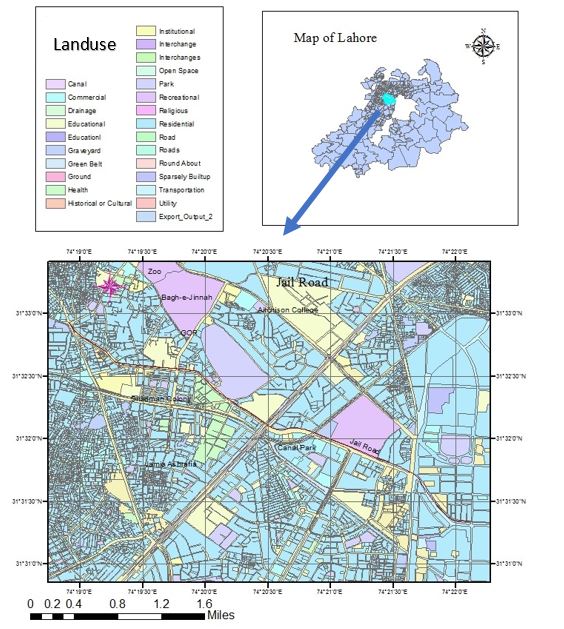
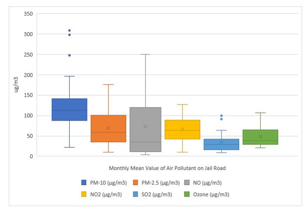
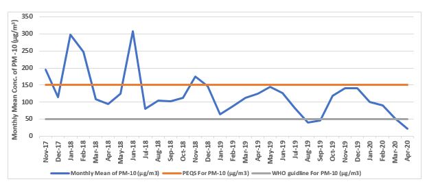
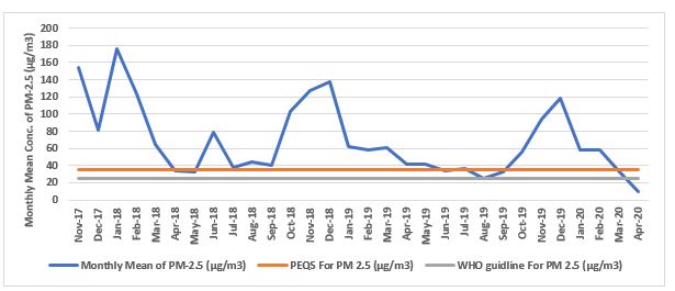
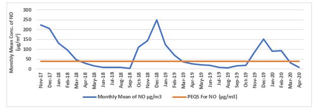
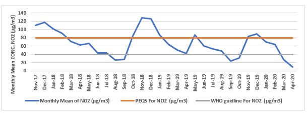
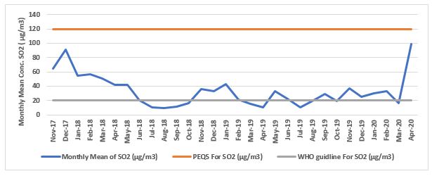
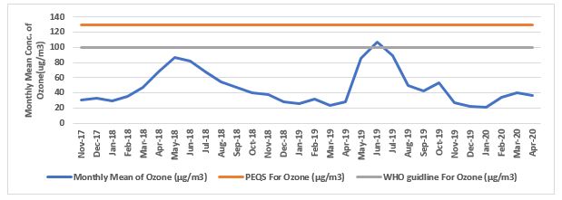
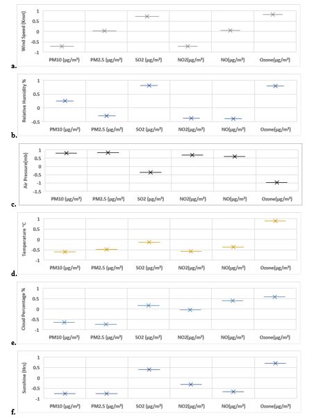
In present study the seasonal prevalence of smog precursors was analysed to investigate the temporal prevalence of air pollutant in the ambient air of Lahore. Data set of three years (November 2017- April 2020) was obtained from compact ambient air quality monitoring station, installed by Environmental Protection Department on Jail Road, Lahore. Statistical analysis of dataset of air pollutant revealed that in winter, the concentration range of PM10, PM2.5, NO, NO2 was significantly higher than Punjab Environmental Quality Standards and WHO Air Quality Guidelines.  while Seasonal impact on air pollutant concentration was further assessed by correlation analysis of weather component with air pollutants. According to statistical analysis, Ozone (O3) was found to have high positive correlation with temperature >wind speed >relative humidity >sunshine hour while inverse relation with air pressure while NO, NO2, SO2, PM2.5 showed positive corelation with air pressure and negative correlation with temperature, sunshine, and wind speed. These factual figures revealed that ambient air of Lahore has been experiencing reducive-type air pollution in winter which is acidic in nature and oxidative-type pollution in summer since 2017 because local weather conditions directly affect the air pollutant transportation behaviour.

Keywords:  Ambient Air; PEQS; Photochemical; Air Pollutant; Smog

Introduction

Diabetes has been increasing in a lot of countries for long, and the number of the patients has reached to 425 million by WHO [1]. It is not only associated with medical problems, but also social and economic problems worldwide. Diabetes contains mac- rovascular complications of brain, heart, lower extremities and microvascular complications such as neuropathy, retinopathy and nephropathy.

As to these diabetic complications, there has been increasing evidence that persisting elevated blood glucose may be responsible for pathological changes [2,3]. Impaired microcirculation would be involved in the etiology of diabetic changes [4]. Regarding the microvascular complications, there seems to be four possible mechanisms influencing the biochemical changes. They are forma- tion of advanced glycation endproducts (AGEs), increased flux of glucose and other sugars through the polyol pathway, activation of protein kinase C (PKC) isoforms and increased flux through the hexosamine pathway [5].

From mentioned above, appropriate measures are crucial to address the problems related to diabetes [6]. As to nutritional therapy of diabetes, Atkins et al. initiated Low Carbohydrate Diet (LCD) [7]. The effect for lowering blood glucose and reducing weight has been recognized broadly. After that, Dietary Intervention Randomized Controlled Trial (DIRECT) Group reported the comparison of effects among low-carbohydrate, Mediterranean and low-fat diet [8,9]. In this case, Low-Fat Diet equals to Calorie Restriction (CR). This brought the discussion about LCD and CR for years [9,10].

On the other hand, authors introduced and developed LCD by seminars in Japan, presenting medical society and medical papers [11,12]. We have also reported clinical study of elevated Ketone Bodies (KB) and its physiological role in the axis of fetus, placenta, newborn and mother [13]. Moreover, we have continued clinical diabetic research concerning LCD and CR [14]. Our recommended three types of LCD have been widely used for patients with type 2 diabetes (T2DM) and obese subjects, including super LCD, mod- erate LCD and petite LCD meals [15].

In this study, we investigated the glucose variability on CR diet by daily profile of blood glucose and M value in patients with T2DM. We also studied clinical effects of LCD for 2 weeks by decreasing blood glucose and M value. Furthermore, we analyzed the rela- tionship among these associated with homeostasis model assessment of insulin resistance (HOMA-R) and homeostasis model as- sessment of β cell function (HOMA-β). The purpose of investigating HOMA-R and HOMA-β would be the study for insulin resistance and secretory ability from pancreas.

Subjects and Methods

In this study, enrolled subjects were 56 patients with T2DM. They were admitted to the hospital for detail evaluation and adequate treatment of T2DM. The subjects were selected by a criterion. Out of many diabetic patients studied, current subjects have the level of immunoreactive insulin (IRI) more than 5 μU/mL, 10 μU/mL and less than 10μU/mL in the fasting morning after overnight fast. The subjects with less than 5 μU/mL, 5 μU/mL and more than 10 μU/mL were excluded in this study.

Regarding the methods, we have had a certain protocol of diabetic evaluation and treatment in our clinical investigation. In current study, the following series of approach were performed.

1. The patients were admitted to the hospital. In the morning of day 2, blood samples were drawn after overnight fasting. The examination included fundamental tests such as lipids, liver and renal function, complete blood count and diabetes related bio- markers. As to diabetes, glucose, HbA1c, IRI, C-peptide, HOMA-R, HOMA-β and M value were measured and calculated.
2. We have made up our diabetic protocol with CR and LCD. As to nutritional therapy, subjects have CR on day 1 and 2, in which the content has protein 15%, fat 25% and carbohydrate 60% with 1400 kcal/day. This ratio is from the standard of the macronutrients recommended by Japan Diabetes Association [16].
3. Subjects have LCD from day 3 to 14 with super LCD meal. The content has 12% of carbohydrate with 1400 kcal/day. We have other two formula, which are standard LCD with carbohydrate 26% and petite LCD with carbohydrate 40%.
4. Several biomarkers were studied in Day 2 and Day 14. In each day, blood samples were drawn in the morning after overnight fasting. Both data were compared in order to investigate the efficacy of LCD during 12 days.

Daily Profile of Blood Glucose

As regard to glucose metabolism, daily profile of blood glucose was studied on day 2 and on day 14. In each day, blood glucose levels were measured 7 times a day and clock times were 08, 10, 12, 14, 17, 19 and 22h. Blood glucose was measured using the Glu test Mint by SKK Sanwa Co. Ltd., Nagoya, Japan. In relation to glucose, HbA1c was measured using the Accu-Chek Aviva Nano (Roche) by Roche Diagnostics, Tokyo, Japan.

After obtaining the data of blood glucose, average blood glucose a day and also the level of Morbus value (M value) were calcu- lated according to the formula equation [17,18].

Morbus value

M value is the biomarker expressing the variability of blood glucose. It indicates two important factors. One is the average blood glucose level in a day, and another is the mean amplitude of glycemic excursions (MAGE) [17-19]. Consequently, M value is a nu- merical value, which means the degree of high blood glucose and the fluctuation of blood glucose. From the mathematical point of view, it is calculated by the logarithmic transformation. The significance of M value means the degree of glucose deviation from the ideal glucose variability [18-20].

M value has three steps for calculation. At first, M=MBS + MW: M value means the total of MBS and MW. In addition, MW means maximum blood glucose − minimum glucose)/20. Further, MBS is the mean of MBSBS. MBSBS is a numerical number for evaluating glucose variability. It is calculated as the absolute value of [10 × log (blood glucose level/120)])3 , which formula is the M value in each BS of | 10 × log BS/120 |3 [18-20].

As to the normal value of M value, the following would be the standard judgment. Clinically, the level of M value would be that it is normal less than 180 is normal range, borderline is from 180 to 320, and abnormal range is more than 320.

Statistical Analysis

As regard to this study, obtained data were shown by mean and standard deviation. In addition, data was described as the median and quartile of 25%/75% according to the necessity of the biomarkers. Boxplot was used for the comparison among some groups, which expresses the median and the quartile of 25%/75%, maximum and minimum. As to investigation for the correlation with biomarkers, we used Spearman test to obtain the correlation coefficients. We utilized JMP (Version 8) statistical analysis software (JMP Japan Division of SAS Institute Japan Ltd.) and Microsoft Excel analytical tool [21].

Ethical Considerations

Current research was conducted in compliance with the ethical principles based upon the Declaration of Helsinki. Moreover, ad- ditional commentary was performed in the Ethical Guidelines for Medical Research in Humans and in accordance with the Good Clinical Practice (GCP), with ongoing consideration to the protection of subjects’ human rights. Furthermore, there was the “Ethical Guidelines for Epidemiology Research” by the Ministry of Education, Culture, Sports, Science and Technology and the Ministry of Health, Labor and Welfare.

consents and written paper agreements have been taken from the subjects. This study has been registered by National University
Hospital Council of Japan (ID: #R000031211).

Results

Fundamental Data

Enrolled subjects (n=56) showed the fundamental data (Table 1). Average age was 63.1 years old with 64 years old in median value. Average or median value of HbA1c and IRI was 7.9% or 7.3% and 7.0 μU/mL or 7.3μU/mL, respectively. Median value of HOMA-R and HOMA-β were 2.63 and 25.9, respectively.

Table 1

Changes in Biomarkers

The changes in biomarkers between day 2 and day 14 were compared as the effect of LCD for 12 days (Table 2). There were de- creased median values of day 2 vs. day 12 in average glucose, M value and triglyceride, which were 181 vs. 139 mg/dL, 60.7 vs. 10.2 and 128 vs. 89.5 mg/dL, respectively.

Table 2

As for the values of average glucose, M value and triglyceride, there were significant difference between day 2 and day 14 (p<0.05) by the statistical investigation using non-parametric tests.

Correlations of M Value

There were significant correlations between M value and also average glucose (p<0.01) and also between M value and HbA1c (p<0.01) (Figure 1). Furthermore, there were significant correlations between M value and HOMA-R (p<0.01) and also between M value and HOMA-β (p<0.01) (Figure 2).

Figure 1

Figure 2

Categorization by M Value

Fifty-six subjects were divided into 4 groups according to the level of M value. Each group has 14 cases, and each group showed the median of M value as 9.5, 44.8, 123 and 346, respectively. The level of M value was remarkably elevated in group 1.

Comparison of Biomarkers in 4 Groups

Median values of blood glucose in 4 groups are 123 mg/dL, 167 mg/dL, 198 mg/dL and 272 mg/dL, respectively (Figure 3A). Me- dian HbA1c values of 4 groups are 6.4%, 6.9%, 7.6%, and 9.7%, respectively (Figure 3B).

Figure 3

Regarding HOMA-R and HOMA-β, the value of each group was calculated. Median values of HOMA-R in 4 groups are 2.3, 2.6, 2.2 and 3.5, respectively (Figure 4A). Median values of HOMA-β in 4 groups are 46.1, 40.7, 24.3 and 15.9, respectively (Figure 4B). The level of HOMA-β decreased from group 1 to 4.

Figure 4

Figure 5

Correlation between M Value and HOMA

The changes in M value between day 2 and day 14 are shown in Figure 5. In 4 groups, the M value decreased from day 2 to day 14. The degree of decrease showed larger in the order of group 1 to 4.

Discussion

In recent years, therapeutic procedure for diabetes has been in focus from various points of view. Some management principle and way for diabetes have been proposed by International Diabetes Federation (IDF), American Diabetes Association (ADA) and American College of Physicians (ACP) [22-24]. One of the controversy points was found concerning the recommended HbA1c in some situations. Consequently, adequate control of glucose variability would be crucial and on discussion [25].

In this study, we examined T2DM cases with fasting IRI greater than 5, 10 and less than 10. As a comparative study, we have our unpublished data, in which IRI was 5 or less. Comparing the ranges of numerical values between our data vs. this report, 0-3 vs. 0-7 for HOMA-R and 0-50 vs. 0-90 for HOMA-β. Regarding the correlation with other factors, the distributions of both are rather overlapped in various biomarkers, and obvious differences between the both were not clarified at the moment. However, these results seem to be the basic data in this area for future study.

The average blood glucose level, HbA1c level and TG level decreased with short term of LCD meal. Especially, in Group 4 with high average blood sugar and M value, the reduced degree was to large extent. It has been known that LCD lowers TG level in short term of the LCD [26]. On the other hand, HDL reveals a slight upward trend after several months, while LDL does not show constant direction, which is descending, rising or stable depending on each case [26].

One of the important factors in this study is M value. It is a useful biomarker due to its numerical value indicating both of mean blood glucose and MAGE [17-20]. Further, average glucose can be measured from blood sampling 7 times a day. According to the previous related reports, the results of the comparison between sampling 7 times and 20 times are almost the same [17,27]. Then, both would have compatible data, as well as the results from continuous glucose monitoring (CGM) [27,28].

The correlation coefficient between M value and the mean blood sugar showed extremely high. The reason would be that the calculation method of the M value is using the quadratic equation including the average blood sugar. Regarding the correlation between M value and HbA1c, the dispersion was small when A1c was from 4% to 8%, but the variation was large from 9% to 12% and the reason would be that HbA1c indicates the average of blood glucose levels in recent 1-2 months. In contrast, M value could be widely distributed, because the average and fluctuation of blood glucose is calculated on that day.

As the result, M value and the HOMA-R had a positive correlation, while M value and the HOMA-β had a negative correlation. Among them, the correlation coefficient was higher in HOMA-β. The reason would be that M value includes mean blood glucose and MAGE with close relationship with insulin secretion, and that HOMA-β represents pancreas function.

HOMA has been used as the useful biomarker for diabetes, where fasting blood sugar and fasting insulin were taken into consid- eration at the time of HOMA calculation. In original, HOMA was initiated by Matthews who is mathematician [29]. HOMA is based on the balance between hepatic glucose output and insulin secretion from fasting levels of glucose and insulin [30].

As to clinical significance and implications of HOMA, functions of both ability to secrete insulin and resistance of insulin have been inferred. There are two formulas of HOMA, including HOMA-R and HOMA-β. When the level of HOMA-R elevates, the insulin re- sistance would be elevated. Concerning the standard value of HOMA-R, 1.73 or more indicates the existence of insulin resistance [31]. In the case of current study, data showed HOMA-R more than 1.73, because all cases had fasting IRI more than 5 μU/mL.

On the other hand, HOMA-β has been known as ability for secreting insulin. The standard value would be 100% in western people, and about 70% in Asian people [32].

From mentioned above, high HOMA-R and low HOMA-β were independently and consistently associated with an increased dia- betes risk [33]. Compared the obtained data of HOMA-R and HOMA-β, most subjects in this study did not show normal ranges, suggesting the existence of insulin resistance and decreased β-function.

When dividing the subjects into several groups for further research, there are some options depending on which biomarker is used. The possible biomarkers can be raised such as fasting blood glucose level, HbA1c, average blood glucose level, M value and so on. Among them, from the point of glucose variability, we adopted M value and divided into 4 groups.

The authors have continued various studies concerning CR and LCD so far [12]. When we use fasting blood glucose as dividing biomarker, their levels have overlapped between normal, mild DM and moderate DM. When using HbA1c indicating average condition in 1-2 months, the correlation between HbA1c and blood variability on that day studied would be a little weak. Mean blood glucose represents glucose variability well on the day of examination, while there is another problem of larger blood glucose fluctuation from postprandial hyperglycemia [33].

On the other hand, M value seems to be beneficial for indicating not only average blood glucose, but also MAGE. Furthermore, the numerical level of the M value ranges very wide, from less than 10 to more than 1000. For this reason, M value would be consid- ered advantageous to be able to utilize research studies for investigating the correlation of related biomarkers.

As to the average blood glucose and HbA1c value in 4 groups, their distribution seemed to be rather divided in the former, and rather overlapped in the latter. The median values of HbA1c in 4 groups were increased from group 1 to group 4.

Furthermore, in 4 groups of HOMA-R and HOMA-β, the distribution showed rather scattered in HOMA-R, and rather divided in HOMA-β. These results would suggest the relationship of M value and HOMA-β indicating insulin secretion function, and the re- search direction of these biomarkers in the future [34].

By LCD treatment, M value in the 4 groups showed a decreasing trend from day 2 to day 14. Among them, in Group 1, the numeri- cal value of M value has not so changed. The reason would be due to the calculation way of M value. It becomes minimum result when blood glucose level is 120 mg/dL. For example, M value increases as blood glucose level decreases from 120 mg/dL to 100 mg/dL.

On the other hand, in groups 2, 3, 4, the higher the M value showed at day 2, the greater M value decreased at day 14. From the above, it can be concluded that marked improvement is observed in the M value, indicating the mean glucose level and MAGE by LCD for 12 days.

Concerning the limit of this study, there are some aspects to be considered. In our several studies, subjects showed wider range of fasting IRI [12,33]. Then, this study included the limited cases with 5-10 μU/mL of IRI. We will plan to investigate diabetic patients with IRI more and less of this level. Obtained results would become fundamental and reference data in the future study. Further- more, other biomarkers would be explored as related to these results. They includes serum and urinary C-peptide, the response of glucose and IRI to standard meal, liver, renal function tests and so on [14,35].

Conclusion

In summary, fifty-six patients with T2DM were investigated in this study. Biomarkers including HbA1c, the daily profile of glucose, average glucose, M value, HOMA-R, HOMA-β, decreased glucose and M value on day 14 were measured and correlations among them were investigated. Obtained results suggest that LCD would be clinically effective for T2DM and there would be relationship among them as to glucose variability. These findings would become fundamental data in this research area, and further study would be expected in the future.

Acknowledgement

Regarding current article, some part of the content was presented at annual congress of Japan Diabetes Society (JDS) Conference, Tokyo, 2018. The authors would like to express gratitude all staffs and patients for the cooperation.

1. Gurjar BR, Butler TM, Lawrence MG, Lelieveld J (2008). Evaluation of emissions and air quality in megacities. Atmos Environ. 42: 1593-606
2. IPCC (2014) Mitigation of climate change. Contribution of Working Group III to the Fifth Assessment Report of the Intergovernmental Panel on Climate Change (IPCC) 1454
3. Abas N, Kalair A, Khan N, Kalair AR (2017) Review of GHG emissions in Pakistan compared to SAARC countries. Renew Sustain Energy Rev. 80: 990-1016.
4. Ramanathan V, Feng Y (2009) Air pollution, greenhouse gases and climate change: Global and regional perspectives. Atmos environ. 43(1): 37-50
5. Saltzman ES, Brass GW, Price DA (1983) The mechanism of sulfate aerosol formation: Chemical and sulfur isotopic evidence. Geophys Res Lett. 10(7): 513-516.
6. Bell ML, Davis DL (2001) Reassessment of the lethal London fog of 1952: novel indicators of acute and chronic consequences of acute exposure to air pollution. Environ Health Perspect, 109: 389-94.
7. Mohammadi H, Cohen D, Babazadeh M, Rokni L (2012) The effects of atmospheric processes on Tehran smog forming. Iran J public health 41: 1.
8. Chen R, Zhao Z, Kan H (2013) Heavy smog and hospital visits in Beijing, China. Am J Respir Crit Care Med. 188(9): 1170-1171.
9. Shabbir M, Junaid A, Zahid J (2019). Smog: A transboundary issue and its implications in India and Pakistan. https://www.think-asia.org/handle/11540/9584
10. NAP (2015) Review of the draft interagency report on the impacts of climate change on human health in the United States. Washington, D.C.: National Academies Press https://www.nap.edu/catalog/21787/review-of-the-draft-interagency-report-on-the-impacts-of-climate-change-on-human-health-in-the-united-states
11. Gaffney SJ, Marley NA, Frederick JE (2011) Formation and effects of smog. Environmental and ecological chemistry. In Encyclopedia of Life Support Systems (EOLSS) (Vol. 2).
12. Butt WH (2017) Distributing destruction: Construction, waste and atmospheres in Lahore. City. 21: 614-21.
13. Raza W, Saeed S, Saulat H, Gul H, Sarfraz M, et al. (2020) A review on the deteriorating situation of smog and its preventive measures in Pakistan. J Clean Prod. 123676.
14. Czerwińska J, Wielgosiński G (2020) The effect of selected meteorological factors on the process of" Polish smog" formation. J Ecol Eng. 21(1).
15. PEQS Punjab Environmental Quality Standard (2016) https://epd.punjab.gov.pk/peqs
16. Hameed R, Bhatti NA, Nadeem O, Haydar S, Khan MA (2013) Comparative Analysis of Emissions from Motor Vehicles Using LPG, CNG and Petrol as Fuel in Lahore. JPIChE. 41: 59-66
17. Butt MT, Abbas N, Deeba F, Iqbal J, Hussain N, Khan RA (2018) Study of Exhaust Emissions from Different Fuels based Vehicles in Lahore City of Pakistan. Asian J Chem. 30: 2481-5.
18. Shah SIH, Nawaz R, Ahmad S, Arshad M (2020) Sustainability Assessment of Modern Urban Transport and Its Role in Emission Reduction of Greenhouse Gases: A Case Study of Lahore Metro Bus. Kuwait J Sci. 47(2).
19. Afon Y, Ervin D (2008) An Assessment of Air Emissions from Liquefied Natural Gas Ships Using Different Power Systems and Different Fuels, J Air & Waste Manag Assoc, 58:3, 404-11.
20. PDMA, 2017. Precautionary Measures Against SMOG. http://pdma.gop.pk/node/373
21. Kgabi NA, Mokgwetsi T (2009) Dilution and dispersion of inhalable particulate matter. WIT Trans Ecol Environ. 127: 229-38.
22. Rani B, Singh U, Chuhan AK, Sharma D, Maheshwari R (2011). Photochemical Smog Pollution and Its Mitigation Measures. J Adv Sci Res. 2(4).
23. Griffing GW (1977) Ozone and oxides of nitrogen production during thunderstorms. J Geophys Res. 82(6): 943-950
24. Tecer LH, Süren P, Alagha O, Karaca F, Tuncel G (2008) Effect of meteorological parameters on fine and coarse particulate matter mass concentration in a coal-mining area in Zonguldak, Turkey. J Air & Waste Manag Assoc. 58: 543-52.
25. Park SS, Kim YJ, Cho SY, Kim SJ (2007) Characterization of PM2. 5 aerosols dominated by local pollution and Asian dust observed at an urban site in Korea during aerosol characterization experiments (ACE)–Asia Project. J Air & Waste Manag Assoc. 57(4): 434-443.
26. Uzoigwe JC, Prum T, Bresnahan E, Garelnabi M (2013). The emerging role of outdoor and indoor air pollution in cardiovascular disease. N Am J Med Sci , 5(8): 445.
27. Derwent et al (2016). Interhemispheric differences in seasonal cycles of tropospheric ozone in the marine boundary layer: Observation‐model comparisons. J Geophys Res Atmos.121(18): 11-75
28. Plocoste T, Dorville JF, Monjoly S, Jacoby-Koaly S, André M (2018) Assessment of nitrogen oxides and ground-level ozone behavior in a dense air quality station network: Case study in the Lesser Antilles Arc. J Air & Waste Manag Assoc. 68(12): 1278-300.
29. Houghton et al (2001) Climate Change 2001: The Scientific Basis, Climate Change 2001: 57.
30. Czernecki et al (2017) Influence of the atmospheric conditions on PM 10 concentrations in Poznań, Poland. J Atmos Chem. 74(1): 115-139.
31. Pöschl U (2005) Atmospheric aerosols: composition, transformation, climate and health effects. Angew Chem Int. 44(46): 7520-7540.
32. Rotstayn LD, Lohmann U (2002) Tropical rainfall trends and the indirect aerosol effect. J Clim. 15(15): 2103-2116.
33. Saleem Z, Saeed H, Yousaf M, Asif U, Hashmi F K, Salman M. Hassali MA (2019) Evaluating smog awareness and preventive practices among Pakistani general population: a cross-sectional survey. Int J Health Promot Educ. 57(3): 161-173.
34. Viidanoja J, Kerminen VM, Hillamo R (2002). Measuring the size distribution of atmospheric organic and black carbon using impactor sampling coupled with thermal carbon analysis: Method development and uncertainties. Aerosol Sci Technol. 36(5):607-616.
35. Von Schneidemesser E, Stone E A, Quraishi TA, Shafer MM, Schauer JJ (2010). Toxic metals in the atmosphere in Lahore, Pakistan. Sci Total Environ. 408(7): 1640-1648.